CSE 163 Final Project - part 2

To view part 1, which talks about our shading model and environment mapping, please click here.
To download the Windows executable along with its necessary components, please click here. Please note that it will take the program a little while to load. Simply double click the executable (Scene.exe) to run the project.

In this blog post, we will talk about the improvements made to our project since the last post.

4. Shadow mapping

Shadow mapping is a technique which first renders the scene from the perspective of the light source (in order to obtain depth information of objects in the scene), then renders the scene again from the regular camera perspective and tries to figure out what parts and objects are occluded from the light source by other objects and parts in the scene.

To calculate this, we need to send information about the light perspective matrices when doing our regular scene rendering to be sent to the shaders.

4.1. The depth map

First, we need to render the scene from the perspective of the light source and save this scene to a texture. In order to do this, the following must be done:

• Set up a new frame buffer that only records depth (i.e. its pixels only have bits for the z-buffer set, no bits for the color buffer).
• Set up a new texture
• Bind the texture to the frame buffer
• Set the texture as the render target by telling the frame buffer that the texture is the destination, not source sampler
• Attach the depth component of the frame buffer to the texture by setting the appropriate flags in OpenGL

Since we only need to obtain the depth information, the shaders are extremely simple - just do the regular coordinate space transformations in the vertex shader, but do nothing in the fragment shader (since the vertex shader already sets the fragment depth for us).

The following is the obtained depth map in our scene:

A sphere, a tank underneath, and the ground

It is important to note the following when obtaining the depth map:

• The light perspective matrix must have a large enough range of values in order to record the depth of all objects in the scene, otherwise there will be areas where no depth information can be obtained since the objects don't show up.
• The near and far planes of the light perspective matrix must be carefully selected
• There are a limited number of bits for the depth buffer, so it is hard to precisely record depth if we set the near and far planes to be too far apart (since rgb values range from 0-255, setting the planes too far apart causes values like 0.000091 and 0.000092 to be recorded as the same).
• Setting the near and far planes to both be too small or both be too large causes the scene objects to be clipped, resulting in (again) no depth information

4.2. Shadow calculation

Once the depth map is rendered to a texture, we must save it somewhere. To ensure that no other textures can interfere with this image, the depth map is rendered to OpenGL texture unit 1 (GL_TEXTURE1, as opposed to the default unit 0 or GL_TEXTURE0). In the shaders, this means the sampler must sample from texture unit 1.

For every fragment, the relative position from the light's perspective must also be calculated, so we send the information about the light perspective matrix over to the shaders for calculation.

If the fragment's depth from the light perspective is calculated to be greater than the depth sampled at the same point on the depth map texture, then that means this particular fragment is in something else's shadow, and therefore no lighting will be done on this fragment.

Since the graphics window coordinates range from (-1, -1) at the bottom left to (1, 1) at the top right, but texture coordinates range from (0, 0) at the bottom left to (1, 1) at the top right, a basic remapping of coordinates need to be done prior to sampling from the depth map texture: we simply add 1 to the xy values, then divide them by 2.

The following are various images obtained by doing a shadow mapping calculation on our scene. The first 2 use the familiar Blinn-Phong shading model, while the third image uses the newly introduced Ashikhmin-Shirley shading model (please refer to part 1 of the writeup for more information, since we talked about this shading model in great detail there):

4.3. Shadow Acne

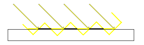
It is clear that there are artifacts that resemble aliasing in our rendered scene. This is due to the fact that because the shadow map is limited in resolution, multiple fragments may sample from the same texel on the depth map. While this can be fixed by increasing the texture image size of the shadow map, it is highly frowned upon as not only does this increase memory overhead, but also does not actually fix anything as the problem will come back if we make our objects even bigger, or if we zoom the camera in a lot.

To fix this issue, a simple workaround is widely adopted: add a small amount of bias to each sampled depth value, so that fragments will not be incorrectly considered to be underneath a surface. This is very much similar to how we have a tolerance value when comparing floating point numbers.

The following diagram from learnopengl.org brilliantly illustrates the problem of why shadow acne exists:

Before showing images of our scene with shadow bias added, we note the following about the bias addition approach:

• The major problem only appears when the light hits the surface at an angle. As a result, we need to zero out the bias when the light is perpendicular to the surface, and a much larger bias as the angle approaches a parallel approach.
• If we do not vary the bias, we get a phenomenon called "peter panning," referring to how the shadows give the illusion that an object is floating slightly above a surface because every single fragment's depth got increased.
• The variance in bias can be easily calculated using the same variables from our direct lighting calculation: we already know the incoming light position, the fragment position, and the surface normal, so we can calculate the bias factor to be the dot product (cosine) of the incoming ray and the surface normal.

4.4 Depth map clipping

While the shadow acne problem has been fixed, it is easy to see that there is a weird fully shadowed zone, and a strange shadow of a tank far away from where it appears. This is attributed to the problem mentioned in section 4.1 about how the light perspective cannot store the information of the whole entire scene. Because textures in OpenGL are defaulted to be repeating, we see that this causes the tank's shadow to appear far, far away, while that whole entire shadowed zone is because it uses the known sampled depth of the ground in the light, but that zone is clearly farther away from the light.

To fix this issue, the following needs to be done:

• Don't check the depth map if the calculated z value is beyond 1, as this is outside of the light's perspective
• This fixes the shadowed region, though it will leave out shadows in some areas - these areas are usually so far away that the user will not notice
• Don't check the depth map if the z value is less than 0, as this is behind the light
• Same note as above
• Change the texture mode to clamp with a value of 1 (no depth information) rather than repeating, when we are outside of the [0, 1] range.

The following images show our scene with this final shadow mapping issue resolved - there is no longer a shadow region in the image:

4.5. More samples

The following are 3 sets of sample side-by-side comparisons of an object with and without shadow mapping. The first image is the Blinn-Phong shading model, while the second and third images use the Ashikhmin-Shirley shading model.

We note that while the Ashikhmin-Shirley shading model does a relatively good job at estimating lighting, the dragon is still lit in unreasonable places, such as the mouth and the legs, which is entirely fixed with shadow mapping.

5. Add-on 2: Extending shadow mapping

For the first add-on, refer to the Ashikhmin-Shirley shading model and the indirect lighting estimation in part 1 of the blog post.

5.1. Multiple lights

Now let us extend this technique for handling multiple lights. In order to do this, we need to set up the following in addition to everything mentioned in section 4:

• Create a brand new depth map for each light in the scene
• This requires generating a new depth buffer ensuring that it gets rendered to a separate texture unit
• The texture unit rendered to must not be used by any other objects that sample from or write to a texture.
• Generate the proper light perspective matrices for each light
• We need to play around with the numbers in order to get a good enough map as mentioned in section 4.1.
• Properly set up and handle multitexturing in the shaders (as the user typically is only able to bind and sample from 1 texture at a time)

Below are some sample images with 2 lights (second light shines in the opposite xz-directions compared to the sun) in the scene:

5.2. Incorrect shadows

While the dragons above now generate shadows for each of the two lights now, we see that the dragons themselves are now much darker. This is because the algorithm falsely sets parts that are not lit by both lights to be in a shadow. This results in most of the models in the scene to be black, since these lights are essentially shining in completely opposite xz directions. For example, for a part that is on the right side of the copper (rightmost) dragon (such as the claw), it is clearly lit by the sun (light 0), but is not lit by the second light (light 1), so the algorithm falsely concludes that it should be shadowed.

A simple fix for this algorithm is proposed as follows:

• Check if a fragment is not lit by both lights. If this condition is true, then it should be black.
• If it is lit by only one light, then ignore the direct illumination from the other light (since it would be 0).
• Otherwise, add up the lighting values for both lights.

This results in a much brighter model, that looks much more realistic than in the previous section:

5.3. Toning the shadows

With the shader and application now able to handle multiple lights, we make one final improvement: make it so that the shadows have varying intensities, depending on how much light it is exposed to. For each light, their shadowing calculation will not return strictly values of 0 or 1, but instead we will change the shadow factor by 1/n, where n is the number of lights, for each light where the fragment is to be occluded. 

While the typical OpenGL application can support up to 7 lights with our extension, it is possible to have up to 79 lights, however we will not do that here as not only will it complicate the memory and calculation overhead, but also very likely bleach out the entire scene because it would be too bright. Instead, we will now add 4 lights to the scene as follows:

With our final improvement to shadow mapping implemented, we now have the following sample gold dragon. The first three images show the dragon shaded by the Blinn-Phong shading model (which, as we know, makes everything look like plastic), and the last two images show the dragon shaded by the Ashikhmin-Shirley model, which makes the dragon actually look like gold. Note the varying intensities of the shadow, both on the ground and on the dragon itself:

It is important to note, however, that the shadows still have very rough edges ("jaggies"). This, as mentioned in section 4.1, is due to the limited resolution available for the shadow map's texture image.

6. Yet another add-on: Non-jagged shadows

6.1. Fixing the jagged edges 

Without increasing the memory overhead of the program, we need to smooth out the shadows in some way. We will therefore perform a fix to the "jaggies" in the shadows as follows:

• In addition to sampling the current texel corresponding to the fragment, we will also sample nearby texels
• Average out the sampled texels

It is important to note the following:

• The scene always has a much higher quality than the depth map texture's resolution, therefore mipmapping the depth map texture does not help. Consequently, bilinear and trilinear filtering cannot be used.
• As a result, we need to perform the neighbor texel sampling approach as mentioned above

The following images now show the same gold dragon as section 5.3, with the add-on applied to the shadows. Note how the shadows appear much smoother now, though the jaggies are still unavoidable once a very high level of zoom is applied. Regardless, we still have a much higher shadow quality than before. As usual, the first two images correspond to the Blinn-Phong shading model, while the second two correspond to the Ashikhmin-Shirley model:

6.2. Sample weighting

Clearly, the neighboring texels contribute the same amount to the final shadow factor calculation. We propose one final modification as follows: weight the texels so that the center texel (corresponding to the fragment itself) has a higher weight, while the neighboring texels have a lower contribution weight. This is very similar to the weight matrix used in project 1, when sharpening images. The weighting used for this project is as follows:

1/25     3/25     1/25

3/25     9/25     3/25

1/25     3/25     1/25

Below are 2 images produced by this weighting scheme. It is important to note that the visual quality does not visually improve - the approach described in the previous subsection is perhaps as good as the algorithm can get:

6.3. More images

Now we add back a shiny ruby dragon, and a dull copper dragon to the scene. The first set of images are the Blinn-Phong shading model (which make them look like shiny plastic), and the second set use the Ashikhmin-Shirley model.

Set 1

Set 2

7. Final touches

7.1. Environment mapping - continued

As you can see, there is only one small issue with the scene: while the environment map does correctly reflect the scene's background, the scene objects themselves (ground, dragons) are not reflected. Consequently, the following must be done:

• Re-draw the scene from the perspective of the center of the reflective sphere
• Use a lower resolution since the sphere is relatively small, and since we need to reduce the program execution overhead.
• Determine the proper texture units and resolutions to render to, otherwise there will be discontinuity or obvious stitching in the skybox
• Clean up the project a little to maintain a high rendering frame rate
• Otherwise it won't be real-time anymore.

With the proper fixes to environment mapping, we have now not only correctly reflected the scene objects, but also their soft shadows. Below are some sample images of this final fix/extension to our project (Ashikhmin-Shirley model only). Note how even the shadow of the reflective sphere itself is also reflected:

7.2. More images

Below is a collection of some fun images, with various different objects placed in it. If the objects look bright and plastic-like, it's more likely than not using the Blinn-Phong shading model. If they look metallic (or dull but not plastic-like), then it's more likely than not using the Ashikhmin-Shirley BRDF model. 

The UCSD stone bear, Blinn-Phong shading

Ditto, with a dull sphere on top

Ditto, with Ashikhmin-Shirley BRDF

Sphere removed from scene

The bear with shadow mapping turned off

A tank and a helpless bunny, Blinn-Phong shading model

Same scene but with Ashikhmin-Shirley BRDF

A different viewing angle

7.3. Scene video

Below is a short video showcasing our scene.

A much higher resolution video is available on YouTube at:
https://youtu.be/qlwN4-wD9FE

This concludes the documentation of the CSE 163 final project.